Vlookup: Learn it, Love it and leave it Part 3 –False Versus True

Data is only as good as the preparation!

  • What happens if we do not force Excel to return the exact data we want?
  • What about looking up an item when there may be more than once instance of it?
  • Troubleshooting data—Can you do it when you are accustomed to using the formula building dialogue box?

To help limit errors we can use three helpful keys to avoid reporting incorrect data:

False versus True
Unique Keys
In Cell / Formula Bar editing versus CTRL+A Dialogue editor

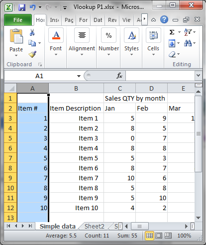
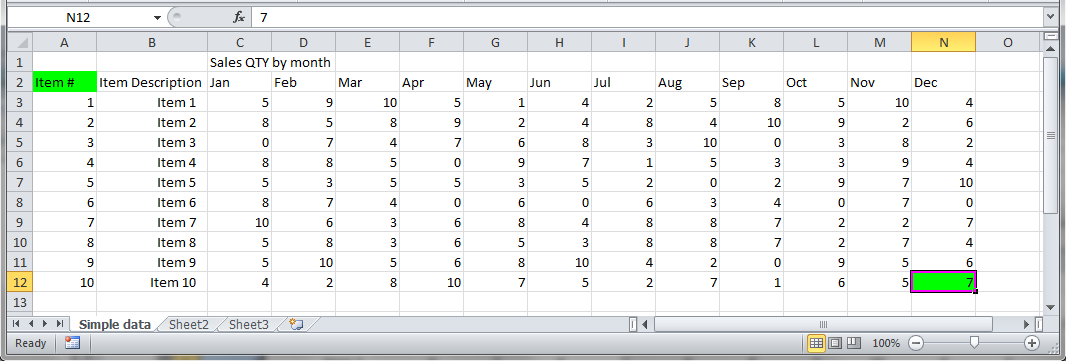
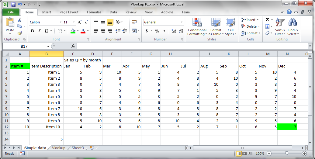
We will discuss False versus True in this post. Download and open this Excel file and follow along.


False versus True:

If you need data integrity, always use False in the [Range_Lookup] section of the Vlookup.

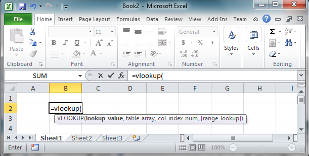
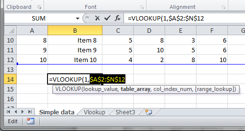
Excel’s formula is broken down as such:

vlookup(Lookup_value, table_array,col_index_num, [range_lookup])

[range_lookup] is bracketed meaning it is optional, yet it determines if the result is exact or a close

True: Returns an approximate match = dangerous when reporting data

Blank: Appears to default to TRUE

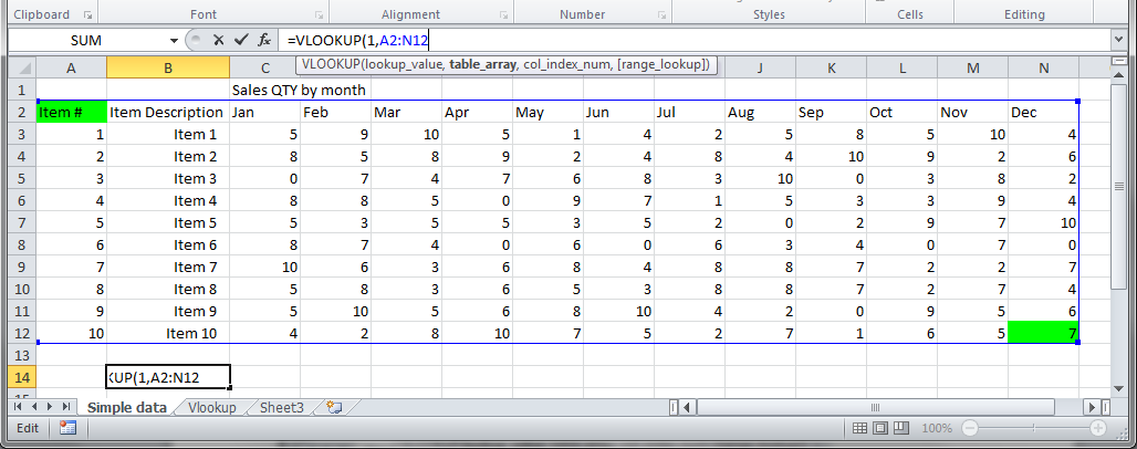
False: Returns data only if the lookup value exists, which runs the risk of a #N/A as a result, and ONLY finds the first instance of the lookup value

Vlookup True False Blank

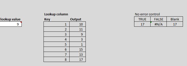
9 is the lookup value. Which output would you report to your boss?

 Why would people use True?

A possible reason includes avoidance of the #N/A result which can disrupt sums, counts and other formulas.

Another is when the source is sorted–you can find something close.

Close / Approximate / Incorrect output could  drastically alter sums, counts, etc.—and the end user doesn’t even know. Which is worse? #NA or incorrect data?

Takeaway: Avoid TRUE unless you have a specific case to use it.

Ideal  formula would look like this:

VLOOKUP(A3,C3:D10,2,FALSE)

To avoid the #N/A add in error control using Iferror or other If statement constructs:

=Iferror(value, value_if_error)

            value_if_error setting:

Null version:   =Iferror(vlookup(A3,C3:D10,2,FALSE),””)

Zero Version:  =Iferror(vlookup(A3,C3:D10,2,FALSE),0)

Adding in Error control cleans the output

Adding in error control cleans the output. I used the “” or Null method to generate a blank. Using Zero may imply a different meaning.

Note:  the method chosen should account for what formulas if any may rely on the output—a null is not the same as a zero when determining averages, counts, etc. Refer to the example Excel file to see the consequences of True/Blank versus False and the Zero versus Null on reporting. Always run sample checks for proper averages, counts etc. Know the question you wish to answer to determine Zero or Null in error control.

IF” constructs (Previous functions work in current versions of Excel):

Pre 2007/10 and forward:

=IF(ISERROR (value))

https://support.office.com/en-AU/article/iserror-function-6a5f3e99-40bc-43ce-a7c8-e79b7b6af5d5

2007/2010 and forward:

=IFERROR(value,value_if_error)

https://support.office.com/en-AU/article/iferror-function-f59bacdc-78bd-4924-91df-a869d0b08cd5

2013:

=IFNA(value, value_if_na)

https://support.office.com/en-au/article/IFNA-function-6626c961-a569-42fc-a49d-79b4951fd461


You are now on your way to sourcing the intended data and not accidentally retrieving unintended data. Look for my next posts on Unique Keys and learning to edit formulas directly in cell or via the formula bar instead of the formula building dialogue box.

Vlookup: Learn it, Love it and Leave it… Part 2 Enhancements

In Part 2, I showed you how to add the dynamic aspects to a Vlookup formula, but we left a lot of room for error. In particular the user may enter data that cannot be found in the data. I showed how entering an “a” for item # failed, likewise the user may wish to enter January, not knowing or realizing Jan is the column header. Part 2 Enhancements shows you how to add validation rules to speed reporting by helping the user enter only what is needed.


Tools to be used: Data Validation.


First we want to be sure that the user only selects valid data.

To do this we will look at our two selections we made Item # and Month in cells C16 and D16. Select cell C16 and then go to:

Ribbon Data tab >> Data Validation >> Validation Criteria >> select List

Click on Data Validation to open the contextual/dialogue box for your inputs:

DataValidation

 In the dialogue box navigate to the Allow: box.

Use selection box by activating the drop down and then select List.

DataValidationList

In Source:  enter the limited range (array) that has all of your items.

Data Validation List Source

For this example we will use the data table itself. In more advanced files we would use a control table to limit our possible items from a master list.

We will enter: $A$3:$A$12.


Once you hit enter, the cell C16 will now show a drop down arrow allowing you to select only what is in the list you referenced.

Data Validated Cell


You can do the same for the Months by selecting cell D16 and applying the list limitation with the source set to $C$2:$N$2. You can either manually type this or select the range with your mouse. Use the Practice tab of the linked file to build your own.


Congratulations, you have now limited the user entries and also helped ensure they are selecting the right items. You are on your way to building reports.

Vlookup: Learn it, Love it and Leave it–Part 1

Vlookup Part 1

Vlookup and the corresponding Hlookup are a new to Excel user’s best friend and over time will become one of your least desired solutions.

Vlookups are used to quickly pull data out of large data tables and are often the go to formula for almost anything an analyst does. Understanding Vlookup is paramount as most Excel users will employ this method extensively and, therefore, you will need to understand what is doing and how to navigate it as well as solve for its limitations.

How the Vlookup works:

When you type in =Vlookup(   in Excel you will be greeted with the formula format:

=vlookup(Lookup_value, table_array,  col_index_num, [range_lookup])

 Vlookup

Of course what this means is obvious to a new user! Great so now what?


Data:

You probably need to find a particular data point.

Likely your team or boss asked you to find how much of item X was sold on date Y in region Z or some other business scenario.  So here you have a lookup item and some limitations. Before we dig deep let’s start with the item lookup.

Assume your company has 10 items and the all sales data is kept in a simple table like below:

(Click here or the image for the sample file to play with housed on Google Drive)

Simple Table

In the table above you have sales quantity data for item#’s one through ten and by month.

To answer your boss’s request your Vlookup formula will need to be limited by which item you need and then which month you need.(For database users the Vlookup is a much like an SQL Select Where statement)

The formula:

vlookup(Lookup_value, table_array,  col_index_num, [range_lookup])

Lookup_value: The selected item you need to find data for

Col_index_num: The column where the date you need data is located

Table_array:  Excel description for the table–its spreadsheet location. We will tackle this in a minute.

[range_lookup]: Set this to False–False returns exact data

Suppose we want Item 1 sales quantity in January. Our Lookup value can be either the Item # or Item Description. As long as we have one of the two we can lookup that item.

Let’s start with the Item # which is in column A. I have the reference column highlighted in the image below.

Selection column

Your data is to the right of column A. Columns are sequential with the first column = 1. We want January data. Jan is column C, which is the 3rd column of the table so the column # = 3.

(Note it is important that you are counting column position from the lookup_value column as a table may not start at column A).


We now know:

Lookup_value is 1

Col_index_num is 3

To complete the formula we need the Table_array.

A table array is the start and stop cells designating the location for the data table. In the table we are using the table starts at cell column A and cell row 2. Excel’s naming convention for cell location is column letter then row # thus A2.

In the below picture I highlighted the tables beginning cell and end cell in green. If you select a cell you will see the cell name populate in the area above the spreadsheet to the left. In this case I will select cell N12. You will also see the column and row indicators highlighted on the edges of the spreadsheet as well as N12 in the left top of the screen.

Table array

To define a range or array we need both the start and end cell names joined together with a colon. Thus this table range is

A2:N12

Notice Excel draws a blue outline around your referenced range:

Blue Box

Note: This range or array reference is referred to as an unanchored range. Some techniques in Excel will cause your unanchored reference to change when using drag, copy/paste, etc. Be sure to check your references.

You may opt for the anchored version which forces the reference to remain unchanged by adding in $ before the column and row indicators like so:

$A$2:$N$12

You can anchor by typing the dollar signs or by pressing F4. You can anchor the column, the row or both, Highlight the A2:N12 and press F4 1 time to anchor both (details for another post as to how, when and why).

 Anchor

Your formula will now look like this:

=VLOOKUP(1,$A$2:$N$12,3,False)

The output of this formula should be 5. Hit enter and you will see the answer:

Answer

Congratulations you have now used the Vlookup. Try one of my next guides to see what you can do with Vlookups!

Please Look at my additional posts as you delve into VLookups:

Part 2

Part 2 Enhancements