In Part 2, I showed you how to add the dynamic aspects to a Vlookup formula, but we left a lot of room for error. In particular the user may enter data that cannot be found in the data. I showed how entering an “a” for item # failed, likewise the user may wish to enter January, not knowing or realizing Jan is the column header. Part 2 Enhancements shows you how to add validation rules to speed reporting by helping the user enter only what is needed.

Tools to be used: Data Validation.

First we want to be sure that the user only selects valid data.

To do this we will look at our two selections we made Item # and Month in cells C16 and D16. Select cell C16 and then go to:

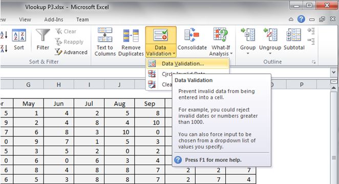
Ribbon Data tab >> Data Validation >> Validation Criteria >> select List

Click on Data Validation to open the contextual/dialogue box for your inputs:

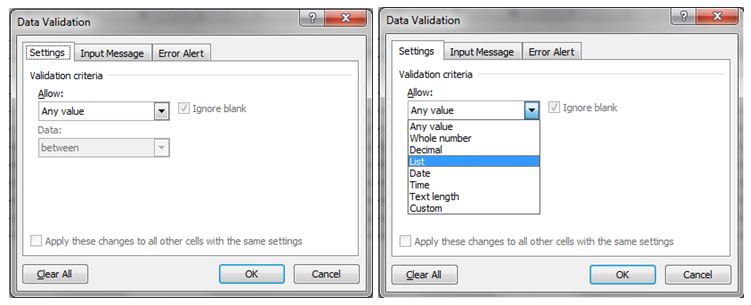
 In the dialogue box navigate to the Allow: box.

Use selection box by activating the drop down and then select List.

In Source:  enter the limited range (array) that has all of your items.

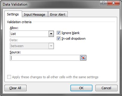
For this example we will use the data table itself. In more advanced files we would use a control table to limit our possible items from a master list.

We will enter: $A$3:$A$12.

Once you hit enter, the cell C16 will now show a drop down arrow allowing you to select only what is in the list you referenced.

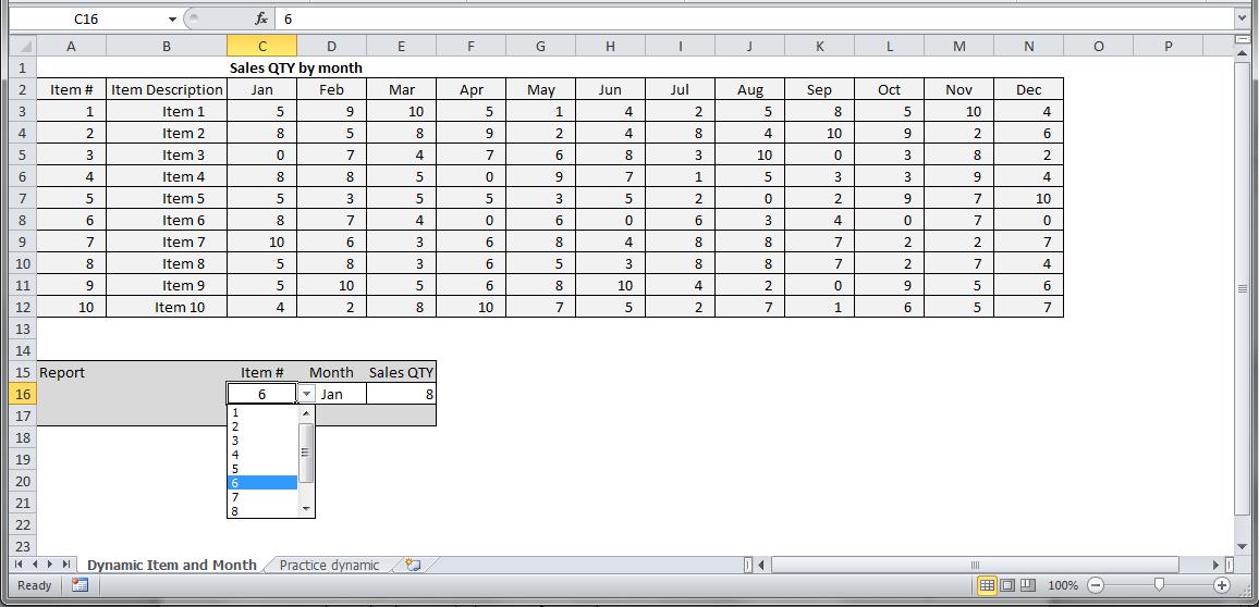
You can do the same for the Months by selecting cell D16 and applying the list limitation with the source set to $C$2:$N$2. You can either manually type this or select the range with your mouse. Use the Practice tab of the linked file to build your own.

Congratulations, you have now limited the user entries and also helped ensure they are selecting the right items. You are on your way to building reports.