A few cents broke my viz!

Posted on October 20, 2017 by alexzbiciak

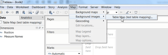
Tableau is a great visualization tool, but as with all software, we must be careful with verifying the results

Applies to:

Extracted data, not Live data

Decimal numbers

Tableau Idea– Please go here and upvote the enhancement

https://community.tableau.com/ideas/8036

Tableau Support

Case: 03336687
Case Description: Decimal 2, fields upon calculation resulting in scientific notation results

Problem statement:

Data from SQL Server set as Numeric Precision 15 and Numeric Scale 2 resulted in a Tableau Extract conversion to Double Precision Float. The conversion led to inaccurate calculation results and a failure during project delivery.

The Story:

During final project delivery — Tableau visualization user acceptance testing — my client identified a handful missing records. The quantity was less than a dozen out of about 200K records — this is not exactly where you want to be. I needed details and fast as we had to deliver. We had to pull out the magnet and find that needle in the haystack…

–I had a hunch–

I asked my developer to send me the records that were identified and what filters and calculations applied to the records in question. And that last one, calculations was the key.

Calculations as Filters–

We were omitting records where a threshold had not been crossed. Tableau said we did not meet the threshold, but the same calculation in SQL Server said we had, as did the client’s original report.

Why?

Bits — Decimals are often not handled well by software — Precision settings matter.

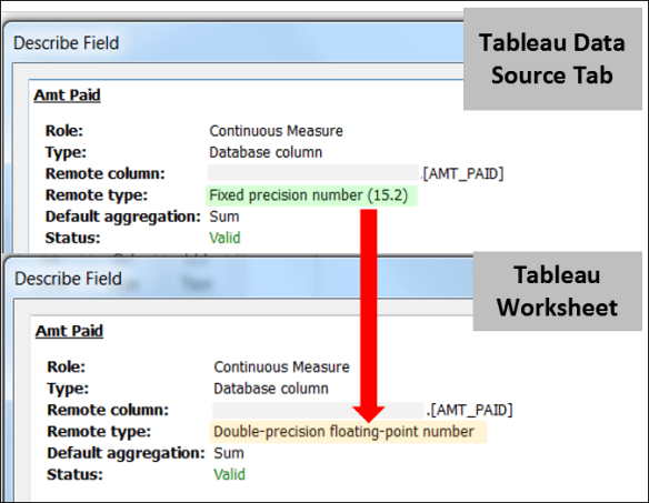
Fixed Precision should inherit to the target –Tableau does not upon extract.

Extraction of SQL Server Fixed Precision 2 decimal field as of 10/20/2017 results in the very different Double Precision Float. The result is some decimal values will be converted to a less accurate value resulting in a potential fractional variances when performing calculations often in the 10-16th decimal place.

Actual Failure At Client:

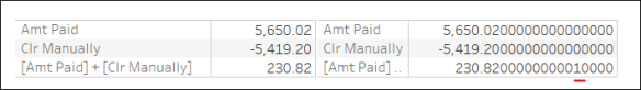
(data selected to simply show decimal value error)

The left side shows the original 2 decimal fields AMT Paid and Clr Manually plus the simple addition calculation [Amt Paid] + [Clr Manually]

To see the Actual value in Tableau Push the decimal values out. The error –> a “1” at the 10th decimal place caused by Double Precision Float binary conversion limitation (likely 32 or 64 bit limit).

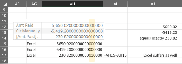
Notice the source fields do not add to the final field value?

If we set a control as either

<= 230.82 or = 230.82

Appears to meet the rule, but will not in a calculation

Reason: The actual value in Tableau is not the original 2 decimal value

The good news:

We were able to deliver the solution — Unfortunately by rounding in the calculation, which I cautioned as a functional, but inaccurate solution.

Testing and Solutions:

Testing with MS Access setting the field definition to currency fixes this when you extract. ***I have not fully vetted this with all possibilities***

I will be updating this with SQL Server testing soon (as time permits)

Tableau Level Workarounds:

Round values
Multiply values by 100, wrap in INT() perform calc, then divide by 100

Datasource workarounds:

MS Access — Currency setting –Note only good for 2 decimal places — Tableau seems to work on extract
SQL server — Money setting (I will be verifying this soon)

What isn’t helped:

Numeric values that must be exactly a specific number of decimals i.e. non-monetary fields or fields with more decimals than monetary fields will accept.

Thanks for reading and be sure to upvote:

https://community.tableau.com/ideas/8036

Tableau Hold ’em — Part 2 — The Flop Card 2

Featured

Posted on October 9, 2017 by alexzbiciak

Remember the need we are trying to answer is: “I want to know if I should bet or not!”

Easiest solution is a YES/NO output, but really?

Welcome to Part 2:

We will

Import your table to Tableau

Map coordinates

Wait! What?

Yes Tableau has a nifty X/Y method that allows you to map out your image and it is a must for this process.

Be sure you have saved your Excel Poker Table as a png ( you can use the Windows Snipping Tool)

YouTube walk-through

1 Create a data set in Excel that you can reference — 3 columns

Position
X
Y

2 Open the Poker Table in Paint and look at the properties

3 Copy the Width and Height in pixels and enter into Excel

Save the Excel file so it can be used as a Tableau Data Source

4 Connect to that data source

5 Open a new worksheet and go to the Map tab at the top of the screen

Select Background images

6 Add your image

7 Place the X/Y pixel counts into the image as X = the right most position and Y = the top most position

8 Create a cross tab with X as column and Y as rows

Things to consider:

In Map >> Background Images be sure you have “Always show Entire Image” selected

Be sure you select “X” and “Y” when you enter your data

You will now see your Texas Hold ’em table

You can hide the headers to make a clean worksheet

Up next –> Tableau Hold ’em Part 3

Previous steps:

https://excelirate.wordpress.com/2017/09/05/tableau-holdem-series/

https://excelirate.wordpress.com/2017/09/18/tableau-hold-em-part-1-the-flop-card-1/

VBA To publish a Batch File from MS Excel

Posted on April 30, 2015 by alexzbiciak

In a previous post I described how to set up a batch file to create a list of files in a directory, specifically MS Excel files.

Sample Excel file with VBA in it.

Question:

Have you ever wanted to bring the data from a set of standardized files into one file using automation?

If so, this blog represents step 2—generating the list remotely. Refer to my previous post to learn how the batch file works.

Tools: MS Excel, MS Windows

Fast Answer–MS Excel VBA Code:

Sub Build_Bat()
'
'''''''''''''''''''''''''''''''''''''''''''''''''''''''''''''''''''''''''''''''''''''''''''''''''''''''''''''''''''''''''
'
' Build_Bat generates a batch file
'
'''''''''''''''''''''''''''''''''''''''''''''''''''''''''''''''''''''''''''''''''''''''''''''''''''''''''''''''''''''''''''

Dim FileNum As Integer
Dim Filepath As String
Dim Folder As String

Filepath = <<Enter your file path here with a closing \>> & "filelist.bat"

'’’’’’’’’’’’’’’’’’’’’’’’’’’’’’’’’’’’’’’’’’’’’’’’’’’’’’’’’’’’’’’’’’’’’’’’’’’’’’’’’’’’’’’’’’’’’’’’’’’’’’’’’’’’’’’’’’’’’’’’’’’’’’’’’’’’’’
'
' Example: Filepath = "C:\Users\Alexander zbiciak\Batch Example\" & "filelist.bat"
'
'’’’’’’’’’’’’’’’’’’’’’’’’’’’’’’’’’’’’’’’’’’’’’’’’’’’’’’’’’’’’’’’’’’’’’’’’’’’’’’’’’’’’’’’’’’’’’’’’’’’’’’’’’’’’’’’’’’’’’’’’’’’’’’’’’’’’’’

'create spot for batch file

FileNum = FreeFile()

'open file

Open Filepath For Output As #FileNum

'write batch file

Print #FileNum, "pushd " & Folder
Print #FileNum, "filetorun -options"
Print #FileNum, "dir /b *.xls? > fileslist.txt"

Close #FileNum

End Sub

Before Macro is run:

After Macro is run:

How To:

First open up Excel and be sure you have the developer tab enabled in your ribbon:

File >> Options >> Customize Ribbon >> Developer

Select the Developer Tab and then the Visual Basic Icon to open your editor:

Inside the editor you will need to add a module if there are none or open one you want to add this code to:

With your module open copy the code below and paste it in (be sure to change your file path):

Sub Build_Bat()
'
'''''''''''''''''''''''''''''''''''''''''''''''''''''''''''''''''''''''''''''''''''''''''''''''''''''''''''''''''''''''''
'
' Build_Bat generates a batch file
'
'''''''''''''''''''''''''''''''''''''''''''''''''''''''''''''''''''''''''''''''''''''''''''''''''''''''''''''''''''''''''''

Dim FileNum As Integer
Dim Filepath As String
Dim Folder As String

Filepath = <<Enter your file path here with a closing \>> & "filelist.bat"

'’’’’’’’’’’’’’’’’’’’’’’’’’’’’’’’’’’’’’’’’’’’’’’’’’’’’’’’’’’’’’’’’’’’’’’’’’’’’’’’’’’’’’’’’’’’’’’’’’’’’’’’’’’’’’’’’’’’’’’’’’’’’’’’’’’’’’
'
' Example: Filepath = "C:\Users\Alexander zbiciak\Batch Example\" & "filelist.bat"
'
'’’’’’’’’’’’’’’’’’’’’’’’’’’’’’’’’’’’’’’’’’’’’’’’’’’’’’’’’’’’’’’’’’’’’’’’’’’’’’’’’’’’’’’’’’’’’’’’’’’’’’’’’’’’’’’’’’’’’’’’’’’’’’’’’’’’’’’

'create spot for batch file

FileNum = FreeFile()

'open file

Open Filepath For Output As #FileNum

'write batch file

Print #FileNum, "pushd " & Folder
Print #FileNum, "filetorun -options"
Print #FileNum, "dir /b *.xls? > fileslist.txt"

Close #FileNum

End Sub

Test your macro by opening the file path in the Windows file explorer. Leave this open so you can watch the VBA output:

With the file explorer window to the side, place your cursor inside the VBA code and then click the play button:

Congratulations—You have now published a batch file from MS Excel.

Vlookup: Learn it, Love it and leave it Part 3 –False Versus True

Posted on March 10, 2015 by alexzbiciak

Data is only as good as the preparation!

What happens if we do not force Excel to return the exact data we want?
What about looking up an item when there may be more than once instance of it?
Troubleshooting data—Can you do it when you are accustomed to using the formula building dialogue box?

To help limit errors we can use three helpful keys to avoid reporting incorrect data:

False versus True
Unique Keys
In Cell / Formula Bar editing versus CTRL+A Dialogue editor

We will discuss False versus True in this post. Download and open this Excel file and follow along.

False versus True:

If you need data integrity, always use False in the [Range_Lookup] section of the Vlookup.

Excel’s formula is broken down as such:

vlookup(Lookup_value, table_array,col_index_num, [range_lookup])

[range_lookup] is bracketed meaning it is optional, yet it determines if the result is exact or a close

True: Returns an approximate match = dangerous when reporting data

Blank: Appears to default to TRUE

False: Returns data only if the lookup value exists, which runs the risk of a #N/A as a result, and ONLY finds the first instance of the lookup value

9 is the lookup value. Which output would you report to your boss?

Why would people use True?

A possible reason includes avoidance of the #N/A result which can disrupt sums, counts and other formulas.

Another is when the source is sorted–you can find something close.

Close / Approximate / Incorrect output could drastically alter sums, counts, etc.—and the end user doesn’t even know. Which is worse? #NA or incorrect data?

Takeaway: Avoid TRUE unless you have a specific case to use it.

Ideal formula would look like this:

VLOOKUP(A3,C3:D10,2,FALSE)

To avoid the #N/A add in error control using Iferror or other If statement constructs:

=Iferror(value, value_if_error)

value_if_error setting:

Null version: =Iferror(vlookup(A3,C3:D10,2,FALSE),””)

Zero Version: =Iferror(vlookup(A3,C3:D10,2,FALSE),0)

Adding in error control cleans the output. I used the “” or Null method to generate a blank. Using Zero may imply a different meaning.

Note: the method chosen should account for what formulas if any may rely on the output—a null is not the same as a zero when determining averages, counts, etc. Refer to the example Excel file to see the consequences of True/Blank versus False and the Zero versus Null on reporting. Always run sample checks for proper averages, counts etc. Know the question you wish to answer to determine Zero or Null in error control.

“IF” constructs (Previous functions work in current versions of Excel):

Pre 2007/10 and forward:

=IF(ISERROR (value))

https://support.office.com/en-AU/article/iserror-function-6a5f3e99-40bc-43ce-a7c8-e79b7b6af5d5

2007/2010 and forward:

=IFERROR(value,value_if_error)

https://support.office.com/en-AU/article/iferror-function-f59bacdc-78bd-4924-91df-a869d0b08cd5

2013:

=IFNA(value, value_if_na)

https://support.office.com/en-au/article/IFNA-function-6626c961-a569-42fc-a49d-79b4951fd461

You are now on your way to sourcing the intended data and not accidentally retrieving unintended data. Look for my next posts on Unique Keys and learning to edit formulas directly in cell or via the formula bar instead of the formula building dialogue box.

Vlookup: Learn it, Love it and Leave it… Part 2

Posted on September 16, 2014 by alexzbiciak

Vlookup Part 2

In Part 1, we learned how to find a data point by declaring a table array or range, using a lookup column and setting which data column we needed to pull data from. That was easy enough, but most data tables are not so easy to use and as an analyst we often require lots of data quickly. To enable quick data retrieval we should employ a dynamic and hopefully scalable method. We must add dynamic abilities to our formulas to speed data capturing for reporting.

Tools:

Tools to be discussed are referencing cells for data and how to isolate the needed columns.

In part 1, we coded our formula to directly look for item 1 using the formula:

=VLOOKUP(1,$A$2:$N$12,3,False)

While this worked great as an Ad-Hoc data lookup, it fails to very be useful. References are hard coded and if using many Vlookups, there will be a lot of downtime to change every formula to generate new results.

Usually analysts need to answer multiple questions and create reports showing lots of data points. Here we will adopt a reference method to allow the formula to become dynamic.

Open and download the Vlookup P2 file to follow along. You will see I added the Report section:

The report section will allow you to change what you are looking up. I like to grey out non-input cells and leave input cells white in my user entry areas. In this case the user can change the Item # and Month. First we will discuss the Item Number reference and how this works.

I selected the item# input cell and you can see Excel references it as C16 in the top left of the screen:

You can use this as your reference id in the Vlookup formula:

Notice the Lookup_value is C16 and Excel color codes the cell reference in the formula and the corresponding cell is outlined in the same color.

The Vlookup formula is now dynamic as to what Item # you can look up. You can enter anything in cell C16, but the formula will only return data for valid references. Try entering 11 or a letter.

Your formula will return the error code #N/A.

Now that we have made the Item selectable, let’s move onto the column. Currently we are using a hard reference for the column (col_index_num).

Our current formula is:

=VLOOKUP(C16,$A$2:$N$12,3,False)

Remember: vlookup(Lookup_value, table_array, col_index_num, [range_lookup])

Although the Col_index_num = 3, we want to make the col_index_num equal to the column position that corresponds to the Month input in Cell D16. Unlike the Item # reference, we cannot just reference Cell D16 for the col_index_num.

A brief discussion of how the C16 reference works:

Using the file linked above:

In any cell type =C16 and you will see the contents of C16 displayed.

In another cell enter =D16 and you will see the contents of D16 displayed. D16 happens to be “Jan” which is the column we want.

Notice, however, that the formula requires a number for the col_index_num, not the Month name. You could enter a number in the Month box, but this may not be the best method. Month #’s will not be the actual column position. Most people would think 1 = Jan, in this case 3 = Jan.

You could write the formula like so:

=VLOOKUP(C16,$A$2:$N$12,D16+2,False)

By using the offset adding 2 you can now select 1 for January and 2 for February, but this is not a good practice as the table may change and the +2 offset is not dynamic—meaning it will not adjust to any changes in the table.

How then will we make the Month selection dynamic? Use the Match function.

=Match(Lookup_value, Lookup_array, [Match_type])

I added a work area to the spreadsheet for trying out the match function:

When using the Match function the function looks through an array and finds if there is a match for you input and then returns the index position, which means the numerical position from start in which the data point was found.

Here we want to find the match for Jan in row 2. Since we are using a text string we have to tell Excel it is text by encapsulating Jan in quotes “Jan”.

Note: Capitalization does not matter in Excel for matching.

Single quotes ‘ in front of data as well as preceding and trailing blank spaces will break a lookup/match so look for these if your data is not coming to you.

Lookup_value will be “jan”.

Lookup_array is 2:2 because the months are found in row 2.

Note: 2:2 is the range of cells that might contain the item we are looking up. This must be a single line or column—unlike a table, you can only reference a single row or single column. To declare the row as a range, you tell Excel it starts in row 2 and ends in row 2 and join the start and stop with a colon, thus 2:2. You can use the anchored version $2:$2.

[Match_type] is optional according to the Excel hint [ ]’s means you can omit for the function to work. To generate the correct output the match_type is very important.

0 = exact match, which is what analysts usually need.

=MATCH(“jan”,2:2,0)

Again a good practice is to anchor your range/array.
.

=MATCH(“jan”,$2:$2,0)

The output of the formula is 3, which tells you the column index position is 3.

We can take the entire match formula and embed it into the vlookup in place of the 3. The new formula will look like this:

=VLOOKUP(C16,$A$2:$N$12,MATCH(D16,$2:$2,0),False)

You now have a fully dynamic lookup formula. Play with the linked file and build your own formulas.

	Stuart Max on Tableau HOLD ’em
	Tableau Hold ’… on Tableau Hold ’em —…
	Tableau Hold ’… on Tableau Hold ’em —…
	Tableau Hold ’… on Tableau HOLD ’em
	Tableau HOLD ’… on Tableau Hold ’em —…

Excel-i-rate

Conquering the data madness

Tag Archives: Report