Data is only as good as the preparation!
- What happens if we do not force Excel to return the exact data we want?
- What about looking up an item when there may be more than once instance of it?
- Troubleshooting data—Can you do it when you are accustomed to using the formula building dialogue box?
To help limit errors we can use three helpful keys to avoid reporting incorrect data:
False versus True
Unique Keys
In Cell / Formula Bar editing versus CTRL+A Dialogue editor
We will discuss False versus True in this post. Download and open this Excel file and follow along.
False versus True:
If you need data integrity, always use False in the [Range_Lookup] section of the Vlookup.
Excel’s formula is broken down as such:
vlookup(Lookup_value, table_array,col_index_num, [range_lookup])
[range_lookup] is bracketed meaning it is optional, yet it determines if the result is exact or a close
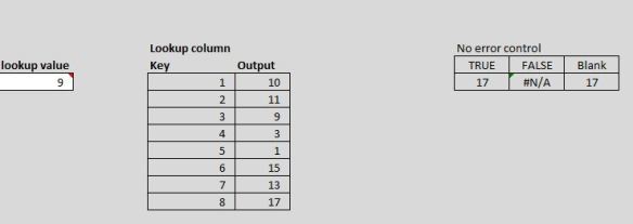
True: Returns an approximate match = dangerous when reporting data
Blank: Appears to default to TRUE
False: Returns data only if the lookup value exists, which runs the risk of a #N/A as a result, and ONLY finds the first instance of the lookup value
Why would people use True?
A possible reason includes avoidance of the #N/A result which can disrupt sums, counts and other formulas.
Another is when the source is sorted–you can find something close.
Close / Approximate / Incorrect output could drastically alter sums, counts, etc.—and the end user doesn’t even know. Which is worse? #NA or incorrect data?
Takeaway: Avoid TRUE unless you have a specific case to use it.
Ideal formula would look like this:
VLOOKUP(A3,C3:D10,2,FALSE)
To avoid the #N/A add in error control using Iferror or other If statement constructs:
=Iferror(value, value_if_error)
value_if_error setting:
Null version: =Iferror(vlookup(A3,C3:D10,2,FALSE),””)
Zero Version: =Iferror(vlookup(A3,C3:D10,2,FALSE),0)

Adding in error control cleans the output. I used the “” or Null method to generate a blank. Using Zero may imply a different meaning.
Note: the method chosen should account for what formulas if any may rely on the output—a null is not the same as a zero when determining averages, counts, etc. Refer to the example Excel file to see the consequences of True/Blank versus False and the Zero versus Null on reporting. Always run sample checks for proper averages, counts etc. Know the question you wish to answer to determine Zero or Null in error control.
“IF” constructs (Previous functions work in current versions of Excel):
Pre 2007/10 and forward:
=IF(ISERROR (value))
https://support.office.com/en-AU/article/iserror-function-6a5f3e99-40bc-43ce-a7c8-e79b7b6af5d5
2007/2010 and forward:
=IFERROR(value,value_if_error)
https://support.office.com/en-AU/article/iferror-function-f59bacdc-78bd-4924-91df-a869d0b08cd5
2013:
=IFNA(value, value_if_na)
https://support.office.com/en-au/article/IFNA-function-6626c961-a569-42fc-a49d-79b4951fd461
You are now on your way to sourcing the intended data and not accidentally retrieving unintended data. Look for my next posts on Unique Keys and learning to edit formulas directly in cell or via the formula bar instead of the formula building dialogue box.


